vii. boundary layer flows the previous chapter considered only viscous internal flows. viscous internal flows have the following major bo
VII. BOUNDARY LAYER FLOWS
The previous chapter considered only viscous internal flows.
Viscous internal flows have the following major boundary layer
characteristics:
* An entrance region where the boundary layer grows and dP/dx ≠
constant,
* A fully developed region where:
• The boundary layer fills the entire flow area.
• The velocity profiles, pressure gradient, and w are constant;
i.e. they are not equal to f(x),
• The flow is either laminar or turbulent over the entire length of
the flow,
i.e. transition from laminar to turbulent is not considered.
However, viscous flow boundary layer characteristics for external
flows are significantly different as shown below for flow over a flat
plate:
Fig. 7.1 Schematic of boundary layer flow over a flat plate
For these conditions, we note the following characteristics:
• The boundary layer thickness grows continuously from the start of
the fluid-surface contact, e.g. the leading edge. It is a function of
x, not a constant.
• Velocity profiles and shear stress are f(x,y).
• The flow will generally be laminar starting from x = 0.
• The flow will undergo laminar-to-turbulent transition if the
streamwise dimension is greater than a distance xcr corresponding to
the location of the transition Reynolds number Recr.
• Outside of the boundary layer region, free stream conditions exist
where velocity gradients and therefore viscous effects are typically
negligible.
As it was for internal flows, the most important fluid flow parameter
is the local Reynolds number defined as
where
= fluid density = fluid dynamic viscosity
= fluid kinematic viscosity = characteristic flow velocity
x = characteristic flow dimension
It should be noted at this point that all external flow applications
will not use a distance from the leading edge x as the characteristic
flow dimension. For example, for flow over a cylinder, the diameter
will be used as the characteristic dimension for the Reynolds number.
Transition from laminar to turbulent flow typically occurs at the
local transition Reynolds number, which for flat plate flows can be in
the range of
With xcr = the value of x where transition from laminar to turbulent
flow occurs, the typical value used for steady, incompressible flow
over a flat plate is
Thus for flat plate flows for which:
x < xcr the flow is laminar
x ≥ xcr the flow is turbulent
The solution to boundary layer flows is obtained from the reduced
“Navier – Stokes” equations, i.e., Navier-Stokes equations for which
boundary layer assumptions and approximations have been applied.
Flat Plate Boundary Layer Theory
Laminar Flow Analysis
For steady, incompressible flow over a flat plate, the laminar
boundary layer equations are:
Conservation of mass:
'X' momentum:
'Y' momentum:
The solution to these equations was obtained in 1908 by Blasius, a
student of Prandtl's. He showed that the solution to the velocity
profile, shown in the table below, could be obtained as a function of
a single, non-dimensional variable
defined as
Table 7.1 the Blasius Velocity Profile
with the resulting ordinary differential equation:
and
Boundary conditions for the differential equation are expressed as
follows:
at y = 0, v = 0 f (0) = 0 ; y component of velocity is zero at y =
0
at y = 0 , u = 0 ; x component of velocity is zero at y = 0
The key result of this solution is written as follows:
With this result and the definition of the boundary layer thickness,
the following key results are obtained for the laminar flat plate
boundary layer:
Local boundary layer thickness
Local skin friction coefficient:
(defined below)
Total drag coefficient for length L ( integration of w dA over the
length of the plate, per unit area, divided by 0.5 U2 )
where by definition and
With these results, we can determine local boundary layer thickness,
local wall shear stress, and total drag force for laminar flow over a
flat plate.
Example:
Air flows over a sharp edged flat plate with L = 1 m, a width of 3 m
and
U = 2 m/s . For one side of the plate, find: (L), Cf (L), w(L), CD,
and FD.
Air: = 1.23 kg/m3 = 1.46 E-5 m2/s
First check Re:
Key Point: Therefore, the flow is laminar over the entire length of
the plate and calculations made for any x position from 0 - 1 m must
be made using laminar flow equations.
Boundary layer thickness at x = L:
Local skin friction coefficient at x = L:
Surface shear stress at x = L:
Drag coefficient over total plate, 0 – L:
Drag force over plate, 0 – L:
Two key points regarding this analysis:
1. Each of these calculations can be made for any other location on
the plate by simply using the appropriate x location for any .
2. Be careful not to confuse the calculation for Cf and CD.
Cf is a local calculation at a particular x location (including x = L)
and can only be used to calculate local shear stress at a specific x,
not drag force.
CD is an integrated average over a specified length (including any
) and can only be used to calculate the average shear stress
over the entire plate and the integrated force over the total length.
Turbulent Flow Equations
While the previous analysis provides an excellent representation of
laminar, flat plate boundary layer flow, a similar analytical solution
is not available for turbulent flow due to the complex nature of the
turbulent flow structure.
However, experimental results are available to provide equations for
key flow field parameters.
A summary of the results for boundary layer thickness and local and
average skin friction coefficient for a laminar flat plate and a
comparison with experimental results for a smooth, turbulent flat
plate are shown below.
Laminar Turbulent
for turbulent flow over entire plate, 0 – L, i.e. assumes turbulent
flow in the laminar region
where
local drag coefficient based on local wall shear stress (laminar or
turbulent flow region)
and
CD = total drag coefficient based on the integrated force over the
length 0 to L
A careful study of these results will show that, in general, boundary
layer thickness grows faster for turbulent flow, and wall shear and
total friction drag are greater for turbulent flow than for laminar
flow given the same Reynolds number.
It is noted that the expressions for turbulent flow are valid only for
a flat plate with a smooth surface. Expressions including the effects
of surface roughness are available in the text.
Combined Laminar and Turbulent Flow
Flat plate with both laminar and turbulent flow sections
For conditions (as shown above) where the length of the plate is
sufficiently long that we have both laminar and turbulent sections:
* Local values for boundary layer thickness and wall shear stress for
either the laminar or turbulent sections are obtained from the
expressions for (x) and Cfx for laminar or turbulent flow as
appropriate for the given region.
* The result for average drag coefficient and thus total
frictional force over the combined laminar and turbulent portions of
the plate is given by
(assuming a transition Re of 500,000)
* Calculations assuming only turbulent flow can typically be made for
two cases:
1. when some physical situation (a trip wire) has caused the flow to
be turbulent from the leading edge or
2. if the total length L of the plate is much greater than the length
xcr of the laminar section such that the total length of plate can be
considered turbulent from x = 0 to L. Note that this will over predict
the friction drag force since turbulent drag is greater than laminar.
With these results, a detailed analysis can be obtained for laminar
and/or turbulent flow over flat plates and surfaces that can be
approximated as a flat plate.
Figure 7.6 in the text shows results for laminar, turbulent and
transition regimes. Equations 7.48a & b can be used to calculate skin
friction and drag results for the fully rough regime.
(7.48a)
(7.48b)
Equations 7.49a & b can be used to calculate total CD for combined
laminar and turbulent flow for transition Reynolds numbers of 5x10⁵
and 3x10⁶ respectively.
Example:
Water flows over a sharp flat plate 2.55 m long, 1 m wide, with Um/s.
Estimate the error in FD if it is assumed that the entire plate is
turbulent.
Water: = 1000 kg/m3 = 1.02 E- m2/s
Reynolds number:
with ( or 10% laminar)
a. Assume that the entire plate is turbulent
This should be high since we have assumed that the entire plate is
turbulent and the first 10% is actually laminar.
b. Now consider the actual combined laminar and turbulent flow:
Note that the CD has decreased when both the laminar and turbulent
sections are considered.
{ Lower than the fully turbulent value}
Thus, the effect of neglecting the laminar region and assuming the
entire plate is turbulent is as expected.
Question: Since xcr = 0.255 m, what would your answers represent if
you had calculated the Re, CD, and FD using x = xcr = 0.255 m?
Answer: You would have the value of the transition Reynolds number and
the drag coefficient and drag force over the laminar portion of the
plate (assuming you used laminar equations).
If you had used turbulent equations you would have red marks on your
paper.
Von Karman Integral Momentum Analysis
While the previous results provide an excellent basis for the analysis
of flat plate flows, complex geometries and boundary conditions make
analytical solutions to most problems difficult.
An alternative procedure provides the basis for an approximate
solution which in many cases can provide excellent results.
The key to practical results is to use a reasonable approximation to
the boundary layer profile, u(x,y). This is used to obtain the
following:
a. Boundary layer mass flow:
where b is the width of the area for which the flow rate is being
obtained.
b. Wall shear stress:
You will also need the streamwise pressure gradient for many
problems.
The Von Karman integral momentum theory provides the basis for such an
approximate analysis. The following summarizes this theory.
Displacement thickness:
Consider the problem indicated in the adjacent figure:
A uniform flow field with velocity U approaches a solid surface. As a
result of viscous shear, a boundary layer velocity profile develops.
A viscous boundary layer is created when the flow comes in contact
with the solid surface.
Key Point: Compared to the uniform velocity profile approaching the
solid surface, the effect of the viscous boundary layer is to displace
streamlines of the flow outside the boundary layer away from the wall.
With this concept, we define * = displacement thickness
* = distance the solid surface would have to be displaced to maintain
the same mass flow rate as for non-viscous flow.
From the development in the text, we obtain
Thus, the displacement thickness varies only with the local
non-dimensional velocity profile. Therefore, with an expression for u
/ U , we can obtain * = f().
Example:
Given: determine an expression for * = f()
Note that for this assumed form for the velocity profile:
1. At y = 0, u = 0 correct for no slip condition
2. At y = , u = U correct for edge of boundary layer
3. The form is quadratic
To simplify the mathematics,
let = y/ at y = 0,0 at y = dy = d
Therefore:
Substituting:
which yields
Therefore, for flows for which the assumed quadratic equation
approximates the velocity profile, streamlines outside of the boundary
layer are displaced approximately according to the equation
This closely approximates flow for a flat plate.
Key Point: When assuming a form for a velocity profile to use in the
Von Karman analysis, make sure that the resulting equation satisfies
both surface and free stream boundary conditions as well as has a form
that approximates u(y).
Momentum Thickness:
The second concept used in the Von Karman momentum analysis is that of
momentum thickness -
The concept is similar to that of displacement thickness in that is
related to the loss of momentum due to viscous effects in the boundary
layer.
Consider the viscous flow regions shown in the adjacent figure.
Define a control volume as shown and integrate around the control
volume to obtain the net change in momentum for the control volume.
If D = drag force on the plate due to viscous flow, taking the fluid
as the control volume, we can write
- D = ( momentum leaving c.v. ) - ( momentum entering
c.v. )
Completing an analysis shown in the text, we obtain
Using a drag coefficient defined as
We can also show that
where: (L) is the momentum thickness evaluated over the length L.
Thus, knowledge of the boundary layer velocity distribution u = f(y)
also allows the drag coefficient to be determined.
Momentum integral:
The final step in the Von Karman theory applies the previous control
volume analysis to a differential length of surface. Performing an
analysis similar to the previous analysis for drag D we obtain
This is the momentum integral for 2-D, incompressible flow and is
valid for laminar or turbulent flow.
where
Therefore, this analysis also accounts for the effect of freestream
pressure gradient.
For a flat plate with non-accelerating flow, we can show that
Therefore, for a flat plate, non-accelerating flow, the Von Karman
momentum integral becomes
From the previous analysis and the assumed velocity distribution of
The wall shear stress can be expressed as
(A)
Also, with the assumed velocity profile, the momentum thickness can
be evaluated as
or
We can now write from the previous equation for w
Equating this result to Eqn. A we obtain
or
which after integration yields
or
Note that this result is within 10% of the exact result from Blasius
flat plate theory.
Since for a flat plate, we only need to consider friction drag (not
pressure drag), we can write
Substitute for to obtain
Exact theory has a numerical constant of 0.664 compared with 0.73 for
the Von Karman integral analysis.
It is seen that the Von Karman integral theory provides the means to
determine approximate expressions for
, w, and Cf
using only an assumed velocity profile.
Solution summary:
1. Assume an analytical expression for the velocity profile for the
problem.
2. Use the assumed velocity profile to determine the solution for the
displacement thickness for the problem.
3. Use the assumed velocity profile to determine the solution for the
momentum thickness for the problem.
4. Use the previous results and the Von Karman integral momentum
equation to determine the solution for the drag/wall shear for the
problem.
and 7.3 and does not have to be accounted for separately.
VII-16
 TABELA DE QUOTIZAÇÃO – 2021 TABLE OF FEES
  FULL D’AUTORITZACIÓ PER LA RECOLLIDA DE L’INFANT JO …………………………………………………
 C HILDREN AND FAMILY SERVICES
 QUALNET 50 TUTORIAL PART 1 INSTALLATION TODO
 ROZDZIAŁ 4 MAŁGORZATA DĄBROWSKA UNIVERSITIES IN A KNOWLEDGEBASED SOCIETY
 REQUISITOS PARA LA PRESENTACIÓN A DESEMPEÑO DOCENTE 2020
  CCSDS FILE DELIVERY PROTOCOL (CFDP)— NOTEBOOK OF COMMON INTERAGENCY
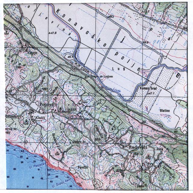 FLOODS IN KARST AREA – CASE STUDY CROATIA